Drawing Smooth Cubic Bezier Curve through prescribed points using Swift
So I wanted to plot some data and decided to create a simple line graph using UIBezierPath. It worked but I wasn’t happy with it. Then I decided to use the quadratic bezier curve method that requires two end points and one control point. Still wasn’t happy with result. Then came the turn of the Cubic bezier curve, that requires two control points and two end points. I knew I needed to use this to create a curve that went through the prescribed points and also creates the smooth and perfect curve that I was looking for. However, it isn’t as straight forward as it first seems.
The bezier cubic curve method signature is this:
func addCurve(to endPoint: CGPoint, controlPoint1: CGPoint, controlPoint2: CGPoint)It requires the next end point, and then two control points. I have the end points (calculated from the data set) but not the control points. This is where my research started. I wanted to figure out how to calculate the control points of a cubic bezier and de Casteljau curve.
Before I get into the algorithm, maths and the code, I would like to say that this article will be far more theoretical and mathematical than any other article that I have posted on this website. It will contain the coding bit as well, but that will be pretty straight forward once you understand the actual logic behind calculating control points. You will need some understanding of Calculus and Linear Algebra.
Now let’s focus on how a bezier curve is actually formed. A quadratic bezier curve has two end points and one control point. The control point can be pictured as a magnet that pushes the main line towards itself giving us the “curve” that we want.
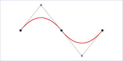
As you can see we have the gray colored point that is basically acting as the control point. To go further in detail, the control point is connected to the two end points. The two lines projecting from the control point are tangent to the curve. Moving the control point will change the gradient of the two lines in turn changing the curve.
But you may ask, how does it actually work? Like it’s not actually a magnet right? Obviously, it’s not a magnet - basically we have simple coordinate geometry going on here. Let’s find out:
The two lines that are projecting from the control point and in tangent to the two end points. Now let’s take a parameter say t which goes from 0 to 1. Also, we will picture that there is a point on each of these gray lines. We will call them p01 and p12. The p01 is moving from endpoint p0 to control point p1 as t goes from 0 to 1. And similarly, we have a point p12 that moves from control point p1 to end point p2 and t goes from 0 to 1.
Imagine there is a line drawn between the point p01 and p12 and there is another point on this line p012. This point moves from p01 to p12 as t goes from 0 to 1. So now when you start the t parameter, you will see that are curve is drawn with respect to the position of the control point.
This is just the basic concept of how bezier curves are formed using one control point. The problem with the quadratic control point is that it only gives us one control point and it doesn’t provide us with the flexibility that we are looking for to create a smooth curve. This same understanding can be applied to cubic bezier curve as well that contains two control points.
To better understand how the bezier curve is drawn, take a look at this extremely well made video/animation:
The Equation:
Now that we have the basic understanding of how bezier curves work, and can picture how the curve is drawn, now it’s time to represent this entire thing with a mathematical equation and here it is:
 (Eq 1)
This is the parameterized equation of a cubic bezier curve, where t which is the parameter can go from 0 to 1. In this equation, the point p0 and p3 are the end point and the point p1 and p2 are the control points. Also note that when t = 0, the output of the equation is p0 and when t = 1, the output is p3. Now as you move the t from 0 to 1 (say in 0.1 increments), the control point contains more weightage in the output. Till a certain t one control point has more weightage and effects the curve more, and for some other range of values for t, the next control point has more weightage and effects the curve.
For example, when t = 0.3:

when t = 0.7, the second control point and the second end point has the most weightage in the curve:

Now let’s take a closer look at how to create smooth curves. The first thing we need to observe is that while this above equation is a 3rd degree polynomial, we can use higher degree polynomials as well which of course means more control points and much precise curve control.
Number of control points = degree of polynomial - 1
However, higher polynomial degree means more complex computations. Therefore, we will stick with 3 degree polynomial or cubic curve. In order to get a long curve, we will stitch cubic curves together.
Conditions:
Since multiple curves will be stitched together, they need to follow a certain protocol:
- Each curve will have two end points (
p0&p3) and two control points (p1&p2). - The last endpoint of one curve will be first endpoint of the next curve. (shared point)
- To get a smooth curve we need to make sure the slope of the line connecting
p2andp3of the curve is same as the slope of line connectingP3andQ1of the next curve.
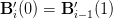
Let’s talk about the derivatives now. The first derivative of any polynomial curve is it’s slope or the gradient at a particular point. The second derivative of the equation tells us about the maxima/minima and continuity behavior. We will use these derivatives to derive equations for our curve. Let’s take a closer look at the third condition of the protocol.
The slope of the line connected p2 and p3 - which is the second control point and last end point of curve should be same as the slope of line connecting the control point Q1 and end point P3. Let’s first write the derivative of the cubic bezier equation:
 (Eq 2)
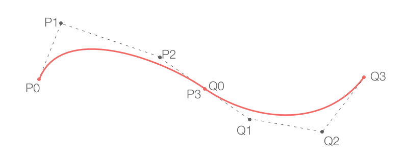
Now before we go any further let’s talk about the segments and points. If you have n data points, and you wish to create a curve that pass through all the data points, then you shall have n - 1 segments or curves. In the above picture you can see that there are three data points, p0, p3 and Q3 and there are 2 curves or segments (from p0 to p3 and from p3 to Q3).
The two curves have a shared point (p3) and we need to make sure that the slope for both curves at this point is same. Note that p3 is the last endpoint for the first segment and the first end point of the next segment.
As I showed earlier in the article, if we put t = 0 in the cubic bezier equation we get the first endpoint as the output and t = 1 yeilds the last endpoint. Similarly, in the Eq 2 (derivative equation of the cubic bezier curve) - we will put t = 1 for the i - 1th segment and t = 0 for the ith segment, where (i > 0).
 (Eq 3)
Once you have substituted the correct t values in Eq 2 and evaluated Eq 3 you will get this equation:
 (Eq 4)
Do note here the second condition of our protocol, that states that the last endpoint of one curve will be first endpoint of the next curve. So point p0 of i segment and point p3 of i - 1 segment are shared or same. We will call them as k. k from now on will represent an endpoint which is shared between two segments.
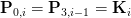
Using the above identity in Equation 4 gives us the following important equation:
 (Eq 5)
We will now move to the second derivative. The second derivative tells us about the continuity of the curve. The second derivative of the bezier curve is:
 (Eq 6)
The second derivative tells us if there is any discontinuity at a particular point in our graph. Since the third condition in our protocol mentions that the curve is continuous so the second derivative shall also be same at the shared point. So go ahead and substitue t = 0 and t = 1 in Eq 6. Make sure that you follow the same concept which was followed earlier:
Substitute t = 0 for the i th segment and t = 1 for i - 1 th segment in the Eq 6 and make them equal to each other. This is what you will get after simplification:
 (Eq 7)
This is our first of three equations which we will use to do most of our evaluation. Also keep in mind that the above equation is in terms of P2 and P1 - the two control points.
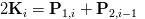
Now we will take a look at the extremities - where the curve starts and ends. These two points have a discontinuity or the second derivative of the curve at these points is 0. Let’s begin by taking the very first segment of the curve. Since the extreme point is when t = 0, so we will substitute t = 0 in Eq 6.
![]()
In the above equation you can see we have P0 which is an end point and not the control point, so we will substitute it with K0 and this is the equation we will get now:
 (Eq 8)
Let’s do the same with t = 1 now for the last segment which will be n - 1 th segment, again make sure to substitute Kn in place of P3 which is an extreme end point of the last segment.
 (Eq 9)
We are almost there. Here is the situation right now: Using our understanding of basic calculus and a bit of algebra, we have been able to get three equations in terms of the unknowns which are the control points P1 and P2. We will first try to solve for one control point and then once P1 is found, we can find P2. So in Eq 7, Eq 8 & Eq 9 we have P1 and P2. We will now get all these three equations in terms of P1 and the K - (which is nothing but the known end points for relative segments).
In order to get this sort of an equation, we will substitute P2 with Eq 5 and we will get the following 3 equations:
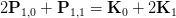 (Eq 10.1)
 (Eq 10.2)
 (Eq 10.3)
The Equations:
The Eq 10.1, 10.2 & 10.3 are the three mains equations that we be using. The equations are in the form of P1 which is unknown and K which is just the end point. Now keep this in mind that the total number of equations will obviously depend on the number of data points. The number of equations will be same as the number of segments or total data points - 1.
Equation 10.1 is the equation to find the P1 of the first segment. Similarly, Equation 10.3 is to find the P1 for the last segment (n - 1). The equation 10.2 is the generic equation, and the quantity of this equation will depend upon the data set. Let’s take a closer look at Eq 10.2.
Equation 10.2 In Depth:
The Equation 10.2 is the most important one when it comes to understanding the whole applied mathematics point of view. We have a system of equations and we will be using a bit of linear algebra to solve for the unknowns.
The i subscript in this equation refers to the index of the data point. For example, i = 0 means, the first element in data array and i = 1 means the second element of the data array. If i = 0, we will use the first equation (10.1), when the i = n - 2, this means we are dealing with second last data point in our array and so we will use the equation 10.3. For i = 1 all the way till i < n - 2, we will use equation 10.2. Confused? Let’s clear it up:
Imagine we have an array p, that contains 7 data points:
let p = [(6,5), (4,2), (7,4), (6,8), (7,1), (8,9), (10,3)]Fetching first data point is pretty trivial = p[0] -> (6,5).
Since in our above equations, we require data points for the right hand side only where Ki is the data point from the array. When we are dealing with first equation (10.1), we need the first and second element of the data set; i = 0 & i = 1.
var p0 = p[0]
var p3 = p[1]
Then for the last segment we need the second last element from the data point, the i value to fetch this will be i = n - 2 or i = 7 - 2 = 5.
 var p0 = p[5]
 var p3 = p[6]
Now, we will use the second equation and our i value will go from i = 1 to i = 4, which returns us the second element till the fifth element:
 for i in 1...4 {
   var p0 = p[i]
   var p3 = p[i + 1]
}
The above example should help us when we are coding this whole thing up.
The Matrix
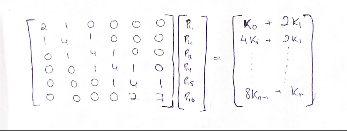
Now is the time to create a matrix where we will use the above equations and create a tri-diagonal matrix. For this example we will assume that we have 7 points, so the total segments will be (7 - 1) = 6. Which means our matrix A will be 6 x 6. Let’s start with Eq 10.1 and Eq 10.3 first:

(M1.0)
We are only concerned with the left hand side of the equations for now.
Now let’s begin adding the remaining elements. The remaining elements will be filled by using the Eq 10.2. The picture below shows the full tri-diagonal matrix:

The tridiagonal matrix essentially contains three diagonals, one main diagonal and then one on top and one on the bottom of the main diagonal. Such matrices are quite easy to compute and takes less computational resources. So now we have the left hand side of the equation. The right hand side is just the data points. Now we will use the Thomas Algorithm to calculate for P1.
A * P1 = B
So this is how our system will look like:
Thomas Algorithm:
Before we get into the coding bit, let’s use the Thomas Algorithm to calculate the unknown P1's. Thomas Algorithm work by working with the three diagonals only and doing simple row operations on them.
The first thing we will do is to make the first element of the main diagonal d = 1.

To do this, we divide first row by d1 and we get:
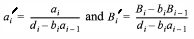
a1' -> a1 / d1
B1' -> b1 / d1
Next, we will use the first row and use it as a pivot to eliminate the element b2:

We do this by multiplying first row with b2 and then is subtracted with the second row, we get:
d2' -> d2 - b2a1'
B2' -> B2 - B1b2
We will do the same operations for all the remaining rows, eliminating essentially the bottom diagonal. So basically we will normalize the second row by dividing the 2nd row with d2' which makes the element d2' = 1. Then we will use this element as the pivot and multiply the entire row with b3 and then is subtracted with the third row, eliminating the b3 element in the below diagonal.
In the end we will get such a matrix:

The last row’s last column is 1, which allows for simple back substitution and finding all the p1's.
Let’s see how we can make all these operations generic, so that we can use a simple for loop and have all these operations take place.
Take three arrays for three diagonals
var d = [Int]
var b = [Int] //below diagonal
var a = [Int] // above diagonal

var B = [Int] // Unknown variable
When i = 1, we will use:
a1' = a1 / d1
B1' = B1 / d1
For i = 2 to i = n - 1:
and when i = n:
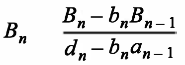
At the end we will do the back substitution to get the values for unknown. We will do this step once we get to the coding portion. Now that we have our P1 control point, we can use these points to get the other control point P2. To get P2, we will use Eq 5 and Eq 9.
If we make P2 the subject we get the following two equations:
 (Eq 11.1)
 (Eq 11.2)
That’s all the maths that we need to do. So now we have the system of equations for P1, and also the equations for P2. Next, we have discussed the thomas algorithm which will help us solve for the system of equations. Now it’s all about the code. The code is pretty straight forward. Let’s code it all out 🚀
Let's Code:
struct BezierSegmentControlPoints {
   var firstControlPoint: CGPoint
   var secondControlPoint: CGPoint
}

class BezierConfiguration {


   var firstControlPoints: [CGPoint?] = []
   var secondControlPoints: [CGPoint?] = []

   func configureControlPoints(data: [CGPoint]) -> [BezierSegmentControlPoints] {


       let segments = data.count - 1


       if segments == 1 {
          // straight line calculation here
          let p0 = data[0]
          let p3 = data[1]

          return [BezierSegmentControlPoints(firstControlPoint: p0, secondControlPoint: p3)]

       }.....
The above block of code basically states that there is a new class called BezierConfiguration that contains a configureControlPoints(data: [CGPoint]) method that takes in an array of CGPointand returns a custom type of BezierSegmentControlPoints that houses the first and second control point per segment.
In side the function, we are first grabbing the total number of segments. If there is just 1 segment or 2 data points, then there will be a straight line and here I am sending the end points as the control points, so in essence there should be no curve on the line.
If segments are more than 1, then we will do the following:
else if segments > 1 {

           //left hand side coefficients
           var ad = [CGFloat]()
           var d = [CGFloat]()
           var bd = [CGFloat]()


           var rhsArray = [CGPoint]()

           for i in 0..<segments {

               var rhsXValue : CGFloat = 0
               var rhsYValue : CGFloat = 0

               let p0 = data[i]
               let p3 = data[i+1]

               if i == 0 {
                   bd.append(0.0)
                   d.append(2.0)
                   ad.append(1.0)

                   rhsXValue = p0.x + 2*p3.x
                   rhsYValue = p0.y + 2*p3.y

               }else if i == segments - 1 { // 5
                   bd.append(2.0)
                   d.append(7.0)
                   ad.append(0.0)

                   rhsXValue = 8*p0.x + p3.x
                   rhsYValue = 8*p0.y + p3.y
               }else {
                   bd.append(1.0)
                   d.append(4.0)
                   ad.append(1.0)

                   rhsXValue = 4*p0.x + 2*p3.x
                   rhsYValue = 4*p0.y + 2*p3.y
               }

               rhsArray.append(CGPoint(x: rhsXValue, y: rhsYValue))

               let solution1 = thomasAlgorithm(bd: bd, d: d, ad: ad, rhsArray: rhsArray, segments: segments, data: data)

               return solution1
           }
In this block of code, we are first creating three arrays, one for the main diagonal d, then one for the diagonal above the main one, ad and one for below, bd. Then we will create a rhsArray that will house all the coefficients for the right hand side of our system of equations. The d, ad and bd will house all the coefficients for the left hand side of the system of equations. Again we are using i to keep track of the index for our original points in the data set. So now we run the for loop that will go from 0 to n - 2 or number of segments - 1.
We need to be careful here not to run a loop where the i is not in the range of the array, so make sure you understand why we are running the for loop till a certain value.
At the start of each iteration, we are calculating the two endpoints for each segment p0 and p3. Then if it is the first point i = 0, then we use the Eq 10.1. we append the respective coefficients to bd, d and ad and the rhsXValue and rhsYValue.
If the index value/ i is equal to segments - 1, or the second last point, then we will append the respective coefficients to the diagonal arrays and also create the rhsXValue and rhsYValue for that equation. Lastly, we have all the segments between the first and last segment. Again we do the same thing and append the coefficients to the diagonals arrays and create the respective rhsXValue and rhsYValue which then we append to the rhsArray.
Thus far, we have created a system of equations. We have the right hand side and left hand side of the equations. Now we will implement the Thomas algorithm. So let’s create a new function and send the relevant data to the function:
func thomasAlgorithm(bd: [CGFloat], d: [CGFloat], ad: [CGFloat], rhsArray: [CGPoint], segments: Int, data: [CGPoint]) -> [BezierSegmentControlPoints] {
In this function, we are getting all the diagonal matrices, the number of segments and the right hand side array and of course our data values. Now we will implement the thomas algorithm. It’s pretty simple and we will just be implementing the equations that we have already discussed earier:
     var controlPoints : [BezierSegmentControlPoints] = [] //Final solution array
     var solutionSet1 = [CGPoint?]()
     solutionSet1 = Array(repeating: nil, count: segments)

       //For the first equation
      ad[0] = ad[0] / d[0]
      rhsArray[0].x = rhsArray[0].x / d[0]
      rhsArray[0].y = rhsArray[0].y / d[0]
The first thing we do inside this function is create a solutionSet1 array and initialize the array with specific number of elements. Next we will solve the first equation, and for that we simply implement the equation already mentioned earlier. The B array that we took in our Thomas Algorithm section will now be replaced with the rhsArray and since we have a point here, so make sure you do the operation to both the x and y coordinates.
Next we will do this for the middle segments or equations. One thing to note here is the fact that we am using the if statement to check if the segments are more than 2. If there are 2 segments only, then we only want the first segment and the last segment code to run.
  //Middle Elements
       if segments > 2 {
           for i in 1...segments - 2  {
               let rhsValueX = rhsArray[i].x
               let prevRhsValueX = rhsArray[i - 1].x

               let rhsValueY = rhsArray[i].y
               let prevRhsValueY = rhsArray[i - 1].y

               ad[i] = ad[i] / (d[i] - bd[i]* ad[i-1])

               let exp1x = (rhsValueX - (bd[i]* prevRhsValueX))
               let exp1y = (rhsValueY - (bd[i]* prevRhsValueY))
               let exp2 = (d[i] - bd[i]* ad[i-1])

               rhsArray[i].x = exp1x / exp2
               rhsArray[i].y = exp1y / exp2
           }
       }
Again we are simplying creating a for loop and iterating through all the remaining rhsArray and diagonals coefficients. Lastly, we will implement the last equation:
//Last Element
      let lastElementIndex = segments - 1
      let exp1 = (rhsArray[lastElementIndex].x - bd[lastElementIndex] * rhsArray[lastElementIndex - 1].x)
      let exp1y = (rhsArray[lastElementIndex].y - bd[lastElementIndex] * rhsArray[lastElementIndex - 1].y)
      let exp2 = (d[lastElementIndex] - bd[lastElementIndex] * ad[lastElementIndex - 1])
      rhsArray[lastElementIndex].x = exp1 / exp2
      rhsArray[lastElementIndex].y = exp1y / exp2
Now, that we have implemented the algorithm, it’s time to do the back substitution. The beauty of this whole Thomas algorithm is that it provides us with the value of the last unknown variable P1(6) and then we will substitute this to the equation above it and keep doing it to find all the unknown. So here we will start with a for loop that is reversed, so it starts with last index value and goes all the way back.
The reason why we initialized the solutionSet1 to nil but with a specific count was so that we can add the last rhsArray element in the last position of the solution set:
solutionSet1[lastElementIndex] = rhsArray[lastElementIndex]for i in (0..<lastElementIndex).reversed() {
let controlPointX = rhsArray[i].x - (ad[i] * solutionSet1[i + 1]!.x)
let controlPointY = rhsArray[i].y - (ad[i] * solutionSet1[i + 1]!.y)
print("CPX", controlPointX, "CPY", controlPointY)
solutionSet1[i] = CGPoint(x: controlPointX, y: controlPointY)
}
firstControlPoints = solutionSet1
So we start a for loop again but reversed, and then find the remaining control points (unknown points) and append it to the solutionSet1 array. Now we have all the first control points. Next we will use the equation 11.1 and 11.2 to find p2.
 for i in (0..<segments) {
           if i == (segments - 1) {

               let lastDataPoint = data[i + 1]
               let p1 = firstControlPoints[i]
               guard let controlPoint1 = p1 else { continue }

               let controlPoint2X = (0.5) * (lastDataPoint.x + controlPoint1.x)
               let controlPoint2y = (0.5) * (lastDataPoint.y + controlPoint1.y)

               let controlPoint2 = CGPoint(x: controlPoint2X, y: controlPoint2y)
               secondControlPoints.append(controlPoint2)
           }else {

               let dataPoint = data[i+1]
               let p1 = firstControlPoints[i+1]
               guard let controlPoint1 = p1 else { continue }

               let controlPoint2X = 2*dataPoint.x - controlPoint1.x
               let controlPoint2Y = 2*dataPoint.y - controlPoint1.y

               secondControlPoints.append(CGPoint(x: controlPoint2X, y: controlPoint2Y))
           }
       }
Now we have two arrays one with all the first control points and the other with second control points. Now we will create any array of BezierSegmentControlPoints where there will P1 and P2 for each segement.
for i in (0..<segments) {
           guard let firstCP = firstControlPoints[i] else { continue }
           guard let secondCP = secondControlPoints[i] else { continue }

           let segmentControlPoint = BezierSegmentControlPoints(firstControlPoint: firstCP, secondControlPoint: secondCP)
           controlPoints.append(segmentControlPoint)
       }

  return controlPoints
UI and Implementation
In the view controller, create an array of data points and instance of UIBezierPath:
  let bezierPath = UIBezierPath()
  let data = [CGPoint(x: 40, y: 150), CGPoint(x: 140, y: 300),CGPoint(x: 230, y: 140), CGPoint(x: 310, y: 250), CGPoint(x: 390, y: 100), CGPoint(x: 490, y: 200), CGPoint(x: 580, y: 270),CGPoint(x: 650, y: 30) ]
In the ViewDidLoad:
override func viewDidLoad() {
    super.viewDidLoad()
    let config = BezierConfiguration()
    let controlPoints = config.configureControlPoints(data: data)
    ...
}
So now we have all the control points. Now after you have grabbed all the control points, start a for loop and create a bezier path:
for i in 0..<data.count {
     let point = data[i]
     if i == 0 {
         bezierPath.move(to: point)
     }else {
         let segment = controlPoints[i - 1]
         bezierPath.addCurve(to: point, controlPoint1: segment.firstControlPoint, controlPoint2: segment.secondControlPoint)
     }
  }
If i == 0, then we will move the bezierPath to that point or in other words start the bezier path. Then for all the remaining points we will grab the segement from the control points array and hen use the addCurve method on bezierPath so provide it with the next point and the control points.
Lastly, we will create the CAShapeLayer and give it some color and animation:
let shapeLayer = CAShapeLayer()
       shapeLayer.path = bezierPath.cgPath
       shapeLayer.lineWidth = 4
       shapeLayer.strokeColor = UIColor.black.cgColor
       shapeLayer.fillColor = .none
       shapeLayer.lineCap = .round
       view.layer.addSublayer(shapeLayer)

       let animation = CABasicAnimation(keyPath: "strokeEnd")
       animation.fromValue = 0.0
       animation.toValue = 1.0
       animation.duration = 2.5

       shapeLayer.add(animation, forKey: "drawKeyAnimation")
And that’s it! We are done 🎉🚀
⭐️ The full project is available on my Github